The Memory Game
The Optimal Strategy for Memory Under Bounded Working Memory
Taulant Koka · March 2026 · GitHub: memory-game
1. The Game
Memory (also known as Concentration or Pairs) is a card game played with $n$ pairs of identical cards ($2n$ cards total), shuffled and placed face down on a table. Players alternate turns. On each turn, a player flips two cards face up. If the two cards match, the player takes the pair and plays again. If they do not match, both cards are flipped back face down and the turn passes to the opponent. The player with the most pairs at the end wins.
Despite being a children’s game, Memory has a surprisingly rich strategic structure. Every card flip reveals information to both players, and the key decision is how to balance learning (flipping new cards) against exploiting what you already know (flipping a card whose match you remember). This raises a natural question: does it matter who goes first?
If you want to skip the theory and just play, there’s an interactive game at the end where you can take on the optimal strategy yourself.
2. What Zwick and Paterson Showed
In 1993, Uri Zwick and Michael Paterson published the definitive analysis of Memory under the assumption that both players have perfect memory: they remember the identity and position of every card ever flipped.
Their key insight was to characterise each game position by just two numbers:
- $n$: the number of pairs remaining on the board
- $k$: the number of cards both players have previously inspected (and remember perfectly)
At each turn, the player chooses one of three moves:
- 0-move (pass): Flip two already-known, non-matching cards. The turn passes to the opponent.
- 1-move: Flip one new card. If it matches a remembered card, take the pair and play again. If not, “waste” the second flip by re-flipping a card you already know.
- 2-move: Flip one new card. If it matches a remembered card, take the pair. If not, flip a second new card. If the two new cards happen to match, take the pair. Otherwise, the turn passes.
Through backward induction on the state space $(n,k)$ (solving the game by working backwards from the end, where the optimal play is obvious, to the beginning), they computed the exact optimal strategy. The results are surprising:
- Player 2 has a slight advantage for even $n \ge 8$, of magnitude about $1/(4n)$ pairs.
- The key strategic weapon is the pass. At high $k$, both players know where most pairs are but deliberately refrain from taking them, engaging in a delicate game of parity control.
- Stalemates occur in a substantial fraction of games under optimal play, when both players pass indefinitely.
This is elegant, but it immediately raises the question: does any of this survive when players do not have perfect memory?
3. First Attempt: Stochastic Memory Decay
My first approach, inspired by Samuel Kilian, was to model forgetting as probabilistic decay: each turn, every remembered card has a probability $\delta$ of being forgotten. This is analytically convenient, the Zwick framework mostly carries over, and it lets you sweep continuously from perfect memory ($\delta=0$) to complete amnesia ($\delta=1$).
I ran large-scale Monte Carlo simulations under this model. The results were interesting: at low $\delta$, the Zwick Player 2 advantage survives. Around $\delta \approx 0.10\text{–}0.15$, there is a phase transition where the Zwick stalemate regime collapses and the game becomes more decisive. At high $\delta$, the game converges to a coin flip.
But the model bothered me. Probabilistic decay means you might remember a card you saw 20 turns ago while forgetting one you saw 2 turns ago. That does not match my experience of how memory works in this game. You either correctly remember where a card is or you do not. And when your brain is full and you see something new, something old gets pushed out. The bottleneck feels more like capacity than reliability.
4. From Miller’s Law to a Tractable Model
This pointed me toward George Miller’s famous 1956 paper on the “magical number seven, plus or minus two”. Later work has revised the effective capacity downward, with Cowan (2001) arguing for something closer to 4 chunks under stricter definitions, and the exact number depends heavily on chunking and task design. For this project I use $M=7$ as a convenient human-scale benchmark, not as a literal psychological constant. The important point is not the precise number but the qualitative fact: working memory has a hard capacity limit, and it is much smaller than a typical Memory board.
Of course, real human memory is more complex than a fixed-size buffer. Decay, interference, attention, emotional salience, rehearsal: they all play a role. A fully realistic model would need to account for all of these, and would almost certainly be intractable.
So I opted for a deliberate simplification: a deterministic bounded-memory model that captures the capacity constraint while remaining analytically solvable. Each player has a working memory of capacity $M$ (number of card positions). When memory is full and a new card is observed, the least recently used entry is evicted.
This is not meant to be a faithful model of human cognition. It is the simplest model that has the property I care about: memory is bounded, and new information displaces old information.
The reason this simplification works so well turns out to be mathematical rather than psychological.
Key property: since both players see every flip and both use the same deterministic eviction rule, both players have identical memory at all times. The memory state is common knowledge. So the game remains one of perfect information, the same class of game Zwick analysed. All that changes is the state space.
Any stochastic model of forgetting (decay, random interference, attention fluctuation) would give the two players different memories, creating private information and turning the game into something closer to poker. That is a much harder problem. The deterministic LRU model sidesteps this and keeps backward induction available.
At the level of the full game, a state consists of:
- the unmatched cards remaining on the board,
- whose turn it is,
- the ordered shared LRU memory list.
The next section shows why, after one key structural theorem, this can be reduced to a much smaller state description.
5. Greedy Matching Is Optimal
Before computing the dynamic program, I need to settle a structural question: if the shared memory already contains both positions of some matching pair, is it ever optimal to leave that pair on the board?
The short answer is no. Under shared memory, if you can see a pair, so can your opponent. Deferring it either hands it to your opponent (who takes it) or risks it being forgotten (evicted from memory). Neither outcome is better than just taking it now.
Theorem
If both players can see a matching pair in shared memory, taking it immediately is always at least as good as any other move.
More precisely: in the bounded-memory model with deterministic LRU eviction, suppose the shared memory contains both positions of some matching pair $P$. Then no legal action that leaves $P$ on the board can yield a higher expected payoff than taking $P$ at once. This is weak dominance: if two pairs are visible simultaneously, taking either one first may be equally good, but deferring a known pair is never strictly better.
Proof
Write $s=(B,\pi,L)$ for a full game state, where $B$ is the set of unmatched cards, $\pi$ is the player to move, and $L$ is the ordered shared LRU memory list. Assume $\pi=A$, and that $L$ contains both $\alpha,\beta$ of the matching pair $P={\alpha,\beta}$.
Let $\sigma$ be any strategy whose first action leaves $P$ on the board. I will construct another strategy $\sigma^+$ that first takes $P$ and then does at least as well.
After taking $P$, the game moves to
\[s^+ := T_P(s),\]which is obtained from $s$ by deleting $\alpha,\beta$ from both the board and the shared memory. The player scores one point and keeps the move.
The only technical point is that deleting a known pair from an LRU memory cannot make the player less able to remember the other unmatched cards.
Lemma (LRU deletion monotonicity). Let $L$ be an LRU memory list, and let $L’$ be obtained from $L$ by deleting some entries. Suppose both lists are then updated by the same sequence of observations
\[x_1,x_2,\dots,x_t,\]none of which is one of the deleted entries. Then deleting entries from an LRU cache cannot reduce recall of the remaining, non-deleted cards. More precisely, after every prefix $x_1,\dots,x_r$:
- every non-deleted card remembered in the original-updated list $L_r$ is also remembered in the deleted-updated list $L’_r$;
- $L’_r$ may additionally remember some non-deleted cards that $L_r$ has evicted, because deleting entries creates spare capacity.
Proof of lemma. Couple the two LRU processes under the same observation sequence. Initially, $L’$ contains all of the non-deleted entries of $L$, and possibly has more free slots. Now process observations one at a time.
If an observed card is already present, the corresponding cache moves it to the MRU end. If it is absent, the cache inserts it and evicts its LRU entry only if full. The deleted cache can never have less effective capacity for non-deleted entries than the original cache, because the deleted entries no longer occupy slots. Therefore an eviction of a non-deleted card in the deleted cache cannot happen before the corresponding eviction in the original cache. Thus a non-deleted card cannot disappear from $L’_r$ while still being present in $L_r$.
The invariant holds for all prefixes. $\square$
Now define $\sigma^+$ as follows. First take $P$. After that, imitate $\sigma$ on the remaining board whenever possible, ignoring any later instruction of $\sigma$ that refers to $P$. This comparison is well-defined because, by the lemma, removing $P$ frees memory slots and does not reduce recall of any other unmatched card under the same future observations.
There are three possible ways the original $\sigma$-line can treat $P$:
Case 1: the opponent takes $P$ before $A$ does. Then $\sigma$ has given the opponent a publicly known pair that $A$ could have taken immediately. The strategy $\sigma^+$ has instead banked that point for $A$ and has not worsened memory for the remaining board. So $\sigma^+$ does at least as well.
Case 2: one of $\alpha,\beta$ is evicted before $P$ is taken. Then $\sigma$ has failed to bank an immediately available point and has allowed the visible pair to disappear from memory. The strategy $\sigma^+$ has already scored that point and has not worsened memory for the remaining board. So $\sigma^+$ does at least as well.
Case 3: $A$ eventually takes $P$. Then both lines eventually give $A$ the same point for $P$, but $\sigma^+$ takes it earlier, keeps the move immediately, and never uses memory capacity to carry the already-known pair. Delaying $P$ creates no additional point and no memory advantage for the rest of the board. So $\sigma^+$ does at least as well.
Thus for every strategy that leaves $P$ on the board, there is a strategy that takes $P$ immediately and yields weakly greater payoff. Therefore leaving a publicly known pair unmatched is weakly dominated, and we may restrict attention to optimal strategies that take such a pair immediately. $\square$
Remark. This proof uses the fact that memory is shared and publicly observable. With private memory, A could know a pair that B does not know about. In that setting, holding the pair in reserve could be genuinely strategic.
Corollary
We may restrict attention to optimal strategies that never leave a publicly known pair unmatched at a decision point. Hence, in reduced states, the shared memory contains only unmatched singletons, one from each of $k$ distinct pairs. The value of a reduced state depends only on $(n,k)$, not on the specific card identities or their LRU order, because all singletons are exchangeable under relabeling. So the game state reduces to the pair $(n,k)$, and the full-state value $V(s)$ becomes the scalar $e_{n,k}$.
Why does value depend only on (n, k)?
Among reduced states with $n$ remaining pairs and $k$ remembered singleton positions, the value depends only on $(n,k)$.
Sketch. Once all remembered cards are unmatched singletons with distinct values, the only quantities that affect the transition law are:
- the number $k$ of remembered singleton positions;
- the number $2n-k$ of unknown positions;
- the number of remembered singleton positions removed or added in each branch.
The specific labels of the remembered cards are exchangeable under relabeling of pair identities. Moreover, when a known card is used as the idle flip in a 1-move or as part of a 0-move, the resulting continuation value depends only on the updated count.
Thus the DP closes on $(n,k)$, and $V(s) = e_{n,k}$ where $(n,k)$ is the reduced state corresponding to $s$.
6. The Optimal Strategy
With greedy matching established, I can compute the optimal strategy by backward induction. The state space is $(n,k)$ where $n$ is the number of pairs left and $k \le \min(n,M)$ is the number of card positions currently in shared memory. At each state, the player chooses between three moves (pass, flip one new card, or flip two new cards) and picks whichever yields the highest expected payoff.
I write $e_{n,k}$ for the value of state $(n,k)$ to the player whose turn it is. Positive means the current player is ahead; negative means the opponent is.
The base cases are straightforward: $e_{0,0}=0$ (no cards left, no points to gain), and $e_{n,n}=n$ whenever $n \le M$ (every remaining pair is known, so the current player takes them all).
Observation convention. When does a flipped card enter working memory? Only when its outcome is unresolved. If a card completes a pair the moment it is revealed, whether by matching the first card (lucky match) or a singleton the opponent recognises (auto-take), the pair is removed immediately and neither card needs to be stored for future recall. Only unresolved cards occupy a memory slot. This convention matters at the boundary $k=M$: a lucky match after one eviction leaves $M-1$ old singletons in memory, not $M-2$.
6.1 The three moves away from the memory boundary ($k \le M-2$)
Let $p = k/(2n-k)$ be the probability that a newly flipped card matches one already in memory, and let $q = 1-p$.
- 0-move (pass): flip two cards you already know don’t match. Nothing changes; the opponent inherits the same state. Value: $0$. Only legal when $k \ge 2$.
- 1-move: flip one new card. If it matches a remembered card (prob $p$), take the pair and play again from $(n{-}1, k{-}1)$. If not (prob $q$), waste your second flip on a card you already know, and the opponent faces $(n, k{+}1)$.
- 2-move: flip one new card. If it matches a remembered card, take the pair. If not, flip a second new card. In this subsection I assume $k \le M-2$, so two unresolved new cards can be stored without eviction.
Full formulas for $k \le M-2$
0-move.
\[e^0_{n,k}=-e_{n,k}.\]Including the pass among the candidate moves is equivalent to clamping the value at zero: if both the 1-move and 2-move are negative, the player passes.
1-move.
\[e^1_{n,k} = p\bigl(1+e_{n-1,k-1}\bigr)-q\,e_{n,k+1}.\]On a match, you score a point and continue with one fewer pair and one fewer singleton in memory. On a miss, the new card enters memory (raising $k$ by one) and the opponent moves.
2-move. Suppose the first card misses. It is now in memory, so there are $k+1$ remembered positions and $d := 2n-k-1$ remaining unknowns. The second card is drawn uniformly from these $d$ unknowns:
- Lucky match (prob $\frac{1}{d}$): the second card matches the first. You take the pair and continue from $(n-1, k)$.
- Auto-take (prob $\frac{k}{d}$): the second card matches a different remembered singleton. The opponent immediately takes that pair, scoring a point and continuing from $(n-1,k)$ in their frame, which is $-(1 + e_{n-1,k})$ in yours.
- Double miss (prob $\frac{2(n-k-1)}{d}$): no match at all. Both new cards enter memory and the opponent faces $(n, k+2)$.
A note on the auto-take bookkeeping: the matched singleton and the second new card are both removed from memory ($-2$), but the first new card stays ($+1$). Net change in $k$: zero. Hence the continuation state is $(n-1,k)$, not $(n-1,k-1)$.
Putting it together:
\[e^2_{n,k} = p\bigl(1+e_{n-1,k-1}\bigr) + q\left[ \frac{1}{d}\bigl(1+e_{n-1,k}\bigr) -\frac{k}{d}\bigl(1+e_{n-1,k}\bigr) -\frac{2(n-k-1)}{d}\,e_{n,k+2} \right].\]6.2 The boundary-adjacent case ($k = M-1$)
There is one extra case between the interior recurrence and the full-memory recurrence. At $k=M-1$, the first missed new card fills the last available memory slot. If the second new card is also unresolved, it must enter memory too, which immediately evicts the least-recently-used singleton. So the double-miss branch goes to $(n,M)$, not $(n,M+1)$.
The 1-move formula is still the ordinary below-capacity formula:
\[e^1_{n,M-1} = p\bigl(1+e_{n-1,M-2}\bigr)-q\,e_{n,M},\]where
\[p=\frac{M-1}{2n-M+1}, \qquad q=1-p.\]For the 2-move, after the first miss the memory is full and there are
\[d=2n-M\]unknown positions available for the second flip:
- Lucky match (prob $\frac{1}{d}$): the second card matches the first. You take the pair and continue from $(n-1,M-1)$.
- Auto-take (prob $\frac{M-1}{d}$): the second card matches one of the old remembered singletons. The opponent takes that pair, and the continuation is $-(1+e_{n-1,M-1})$ in your frame.
- Double miss (prob $\frac{2(n-M)}{d}$): both new cards are unresolved. The second new card enters memory and evicts the LRU singleton, so the opponent faces $(n,M)$.
Thus
\[e^2_{n,M-1} = p\bigl(1+e_{n-1,M-2}\bigr) + q\left[ \frac{1}{d}\bigl(1+e_{n-1,M-1}\bigr) -\frac{M-1}{d}\bigl(1+e_{n-1,M-1}\bigr) -\frac{2(n-M)}{d}\,e_{n,M} \right].\]Equivalently,
\[e^2_{n,M-1} = p\bigl(1+e_{n-1,M-2}\bigr) + q\left[ \frac{2-M}{d}\bigl(1+e_{n-1,M-1}\bigr) -\frac{2(n-M)}{d}\,e_{n,M} \right].\]6.3 What changes when memory is full ($k = M$)
When memory is already full, flipping a new card triggers LRU eviction: the new card enters and the oldest singleton is pushed out. This changes the recurrence in two ways.
First, a miss no longer increases $k$. Instead of advancing to $(n, M+1)$, the state loops back to $(n, M)$. This makes the equations self-referential, but they can still be solved in closed form.
Second, eviction changes the number of unknowns available for the second flip in a 2-move. Below capacity, the first miss turns one unknown into a known card, reducing the unknown count by one (from $2n-k$ to $2n-k-1$). At the boundary, the evicted card re-enters the unknown pool at the same time, so the two effects cancel: the number of unknowns stays at $d := 2n - M$.
After the first miss, memory holds $M-1$ old singletons plus the first new card. Only those $M-1$ old singletons can be matched by the second card (the evicted one is no longer remembered). So the auto-take probability drops from $M/d$ to $(M-1)/d$, and both the lucky-match and auto-take branches lead to $(n-1, M-1)$ rather than $(n-1, M)$.
Full boundary formulas at k = M
1-move at $k=M$. A miss evicts the oldest singleton and loops back to $(n,M)$:
\[e^1_{n,M} = p\bigl(1+e_{n-1,M-1}\bigr)-q\,e_{n,M}.\]If the 1-move turns out to be optimal at this state, then $e_{n,M}=e^1_{n,M}$ and we can solve directly:
\[e^1_{n,M} = \frac{p\bigl(1+e_{n-1,M-1}\bigr)}{1+q}.\]2-move at $k=M$. After a first-card miss (with eviction), the second card is drawn from $d = 2n-M$ unknowns:
- Lucky match (prob $\frac{1}{d}$): the second card matches the first. Take the pair; $M-1$ old singletons remain. The state is $(n-1, M-1)$, not $(n-1, M-2)$, because the second card is acted on immediately and never enters memory (see observation convention above).
- Auto-take (prob $\frac{M-1}{d}$): the second card matches one of the $M-1$ remaining old singletons. The opponent takes that pair. State: $(n-1, M-1)$.
- Double miss (prob $\frac{2(n-M)}{d}$): no match. Memory is still full; the state loops back to $(n, M)$.
Sanity check: $1 + (M-1) + 2(n-M) = 2n - M = d$. $\checkmark$
\[e^2_{n,M} = p\bigl(1+e_{n-1,M-1}\bigr) + q\left[ \frac{1}{d}\bigl(1+e_{n-1,M-1}\bigr) -\frac{M-1}{d}\bigl(1+e_{n-1,M-1}\bigr) -\frac{2(n-M)}{d}\,e_{n,M} \right].\]Collecting $e_{n,M}$ on the left:
\[e^2_{n,M} = \frac{ \left(p+\frac{q(2-M)}{d}\right)\bigl(1+e_{n-1,M-1}\bigr) }{ 1+\frac{2q(n-M)}{d} }.\]Every term on the right involves $n-1$ pairs, which have already been computed. This closed-form boundary equation replaces Zwick’s deep-$k$ recursion.
6.4 Optimal move selection
At each state $(n,k)$, the player picks the move with the highest value:
\[e_{n,k} = \begin{cases} e^2_{n,0}, & k=0,\\[4pt] \max\bigl\{e^1_{n,k},\,e^2_{n,k}\bigr\}, & k=1,\\[4pt] \max\bigl\{0,\,e^1_{n,k},\,e^2_{n,k}\bigr\}, & k\ge 2. \end{cases}\]At $k=0$ there is nothing in memory to match, so the 1-move is unavailable. The pass also requires at least two known cards, so only the 2-move remains. At $k=1$ the pass is still unavailable. For $k \ge 2$ the pass (value $0$) enters the candidate set.
The recursion is evaluated by increasing $n$, and for each $n$ by decreasing $k$ from $\min(n,M)$ down to $0$. This ordering ensures that every value on the right-hand side has already been computed. The only self-referential terms occur at $k=M$, where they are resolved in closed form before computing the boundary-adjacent state $k=M-1$.
Two technical subtleties
Why eviction does not bias match probabilities. One might worry that forgetting cards changes the distribution of what remains. It does not: conditional on the current reduced state, a forgotten card is indistinguishable from one that was never seen. The original shuffle is uniform, and the unseen portion of the board remains exchangeable regardless of eviction history. So the match probability is still $k/(2n-k)$.
Why optimal moves can change even below capacity. Away from the boundary, specifically for $k \le M-2$, the 2-move formula is identical to the corresponding Zwick formula. Yet the optimal move at, say, $k=3$ can still differ between the two models. The reason is that the values plugged into those formulas are different, because they ultimately depend on what happens at the boundary.
An analogy: the riverbed is the same for the first few miles, but Zwick’s river flows on to the sea while the bounded model hits a dam at the memory limit. The dam changes the water level everywhere upstream.
Concretely, $e_{12,3}$ depends on $e_{12,5}$, which depends on $e_{12,7}$. In Zwick’s model, $e_{12,7}$ feeds into $k=8,9,\dots,12$, including the pass equilibrium. Under $M=7$, $e_{12,7}$ is the full-memory boundary state, while $e_{12,6}$ is the boundary-adjacent state whose double-miss branch feeds into $e_{12,7}$. Same local recurrence far enough from the boundary, different downstream values, different optimal move.
7. Results
Move tables
The tables below show the optimal move at each knowledge level $k$ for several board sizes. Bold entries mark where the bounded-memory strategy differs from Zwick.
$n = 8$ (16 cards):
| $k{=}0$ | $1$ | $2$ | $3$ | $4$ | $5$ | $6$ | $7$ | $8$ | |
|---|---|---|---|---|---|---|---|---|---|
| Zwick $(M{=}\infty)$ | 2 | 2 | 1 | 2 | 1 | 2 | 1 | 0 | 1 |
| Bounded $(M{=}7)$ | 2 | 2 | 1 | 2 | 1 | 0 | 1 | 1 | — |
$n = 10$ (20 cards):
| $k{=}0$ | $1$ | $2$ | $3$ | $4$ | $5$ | $6$ | $7$ | $8$ | $9$ | $10$ | |
|---|---|---|---|---|---|---|---|---|---|---|---|
| Zwick $(M{=}\infty)$ | 2 | 2 | 1 | 2 | 1 | 2 | 1 | 2 | 1 | 0 | 1 |
| Bounded $(M{=}7)$ | 2 | 2 | 1 | 2 | 1 | 1 | 1 | 1 | — | — | — |
$n = 12$ (24 cards):
| $k{=}0$ | $1$ | $2$ | $3$ | $4$ | $5$ | $6$ | $7$ | $8$ | $9$ | $10$ | $11$ | $12$ | |
|---|---|---|---|---|---|---|---|---|---|---|---|---|---|
| Zwick $(M{=}\infty)$ | 2 | 2 | 1 | 2 | 1 | 2 | 1 | 2 | 1 | 0 | 1 | 0 | 1 |
| Bounded $(M{=}7)$ | 2 | 2 | 1 | 1 | 1 | 1 | 1 | 1 | — | — | — | — | — |
$n = 16$ (32 cards):
| $k{=}0$ | $1$ | $2$ | $3$ | $4$ | $5$ | $6$ | $7$ | |
|---|---|---|---|---|---|---|---|---|
| Zwick $(M{=}\infty)$ | 2 | 2 | 1 | 2 | 1 | 2 | 1 | 2 |
| Bounded $(M{=}7)$ | 2 | 1 | 1 | 1 | 1 | 1 | 1 | 1 |
$n = 20$ (40 cards):
| $k{=}0$ | $1$ | $2$ | $3$ | $4$ | $5$ | $6$ | $7$ | |
|---|---|---|---|---|---|---|---|---|
| Zwick $(M{=}\infty)$ | 2 | 2 | 1 | 2 | 1 | 2 | 1 | 2 |
| Bounded $(M{=}7)$ | 2 | 1 | 1 | 1 | 1 | 1 | 1 | 1 |
For $n=16$ and $n=20$, the Zwick columns are truncated at $k=7$ for comparison; the full tables extend to $k=n$ with the familiar alternating 2/1 pattern and passes near the top.
A clear pattern emerges as the board grows: the bounded-memory strategy converges to “flip two unknowns only at $k=0$; flip one everywhere else.” The second unknown card mostly churns memory, and the cost of that churn increases with board size.
In practical terms: once you know a few card positions, stop flipping two unknowns per turn. Flip one, keep what you know, and match when you can.
Position values
Expected gain for the starting player (negative = Player 2 advantage):
| $M$ | $n=8$ | $n=10$ | $n=12$ | $n=16$ | $n=20$ |
|---|---|---|---|---|---|
| 3 | $+0.039$ | $+0.030$ | $+0.024$ | $+0.017$ | $+0.014$ |
| 5 | $-0.005$ | $+0.013$ | $+0.018$ | $+0.015$ | $+0.012$ |
| 7 | $-0.007$ | $-0.039$ | $\mathbf{-0.030}$ | $+0.007$ | $+0.010$ |
| 9 | $-0.033$ | $-0.039$ | $-0.020$ | $-0.026$ | $-0.001$ |
| $\infty$ | $-0.033$ | $-0.038$ | $-0.020$ | $-0.018$ | $-0.012$ |
These are exact values computed in rational arithmetic, with no simulation noise. For $n=12$ at $M=7$, the Player 2 advantage is $-0.030$, larger in magnitude than Zwick’s perfect-recall value of $-0.020$.
At very low $M$, memory is too small for strategy to matter and Player 1’s first-mover advantage dominates. At high $M \ge n$, the model recovers Zwick exactly.
8. Simulations
The exact DP gives values and optimal moves, but simulations show how strategies perform against one another and let me explore settings where exact analysis is unavailable, such as fluctuating capacity and asymmetric players.
8.1 Bounded-memory optimum vs Zwick
Both players have $M=7$. I pit the bounded-memory optimal strategy against Zwick’s perfect-recall strategy in all four matchup combinations, across board sizes from $n=8$ to $n=36$.
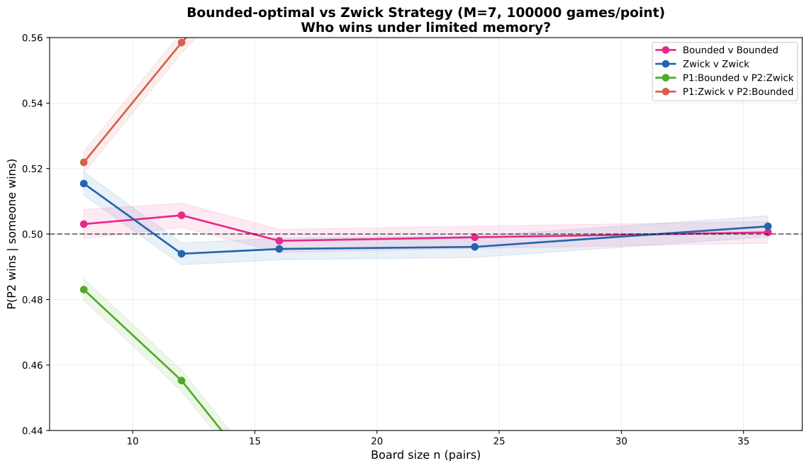
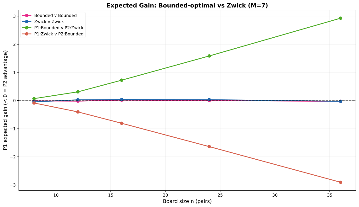
Against opponents using Zwick’s policy, the bounded-memory-optimal policy wins across all tested board sizes. At $n=36$ (72 cards), the bounded-memory player gains roughly 3 full pairs over a Zwick opponent. The gain grows with board size because larger boards spend more time near the full-memory boundary where the two strategies differ.
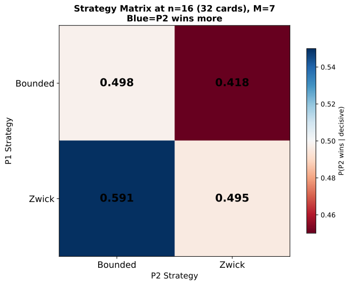
The strategy matrix at $n=16$ shows that bounded-memory optimal dominates Zwick within this two-strategy comparison: no matter which of the two strategies your opponent plays, you are better off playing bounded. (The DP proves optimality within the full class of 0/1/2-move strategies; the simulation confirms it specifically against Zwick.)
8.2 Robustness to fluctuation
Real working-memory capacity is not fixed at exactly 7 every turn. I model this by drawing the effective capacity each turn from $M_0+\mathrm{Uniform}(-\sigma,+\sigma)$, clamped to a feasible range.
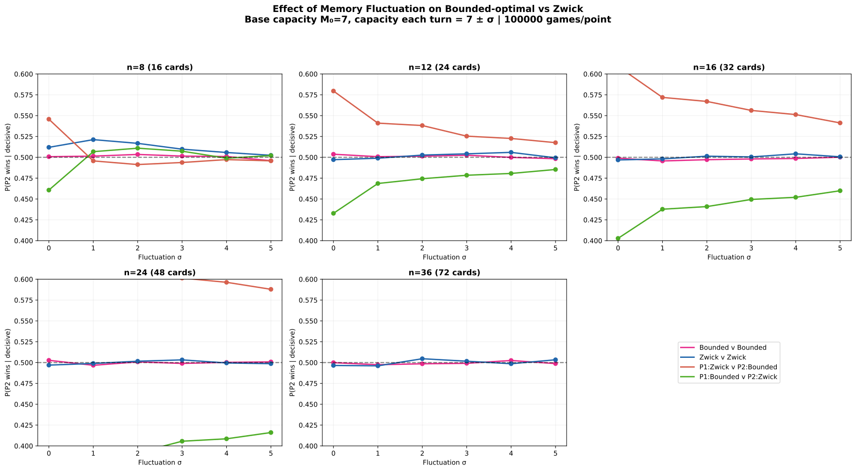
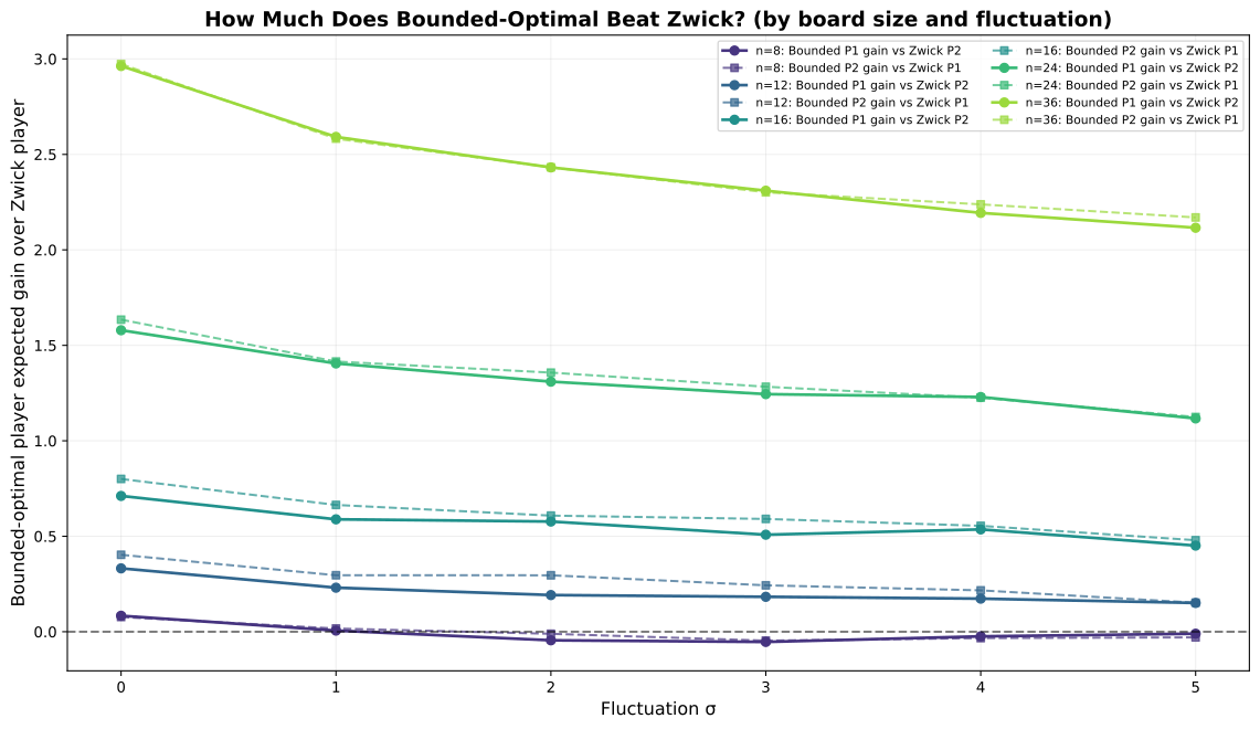
The bounded-memory strategy remains dominant across all fluctuation levels. Even when capacity varies widely, flipping one new card is robust, while Zwick’s two-card exploration remains fragile because it churns memory.
8.3 Asymmetric memory
What happens when the two players have different capacities? Say, an adult ($M=9$) against a child ($M=5$). Each player uses the optimal strategy for their own capacity.
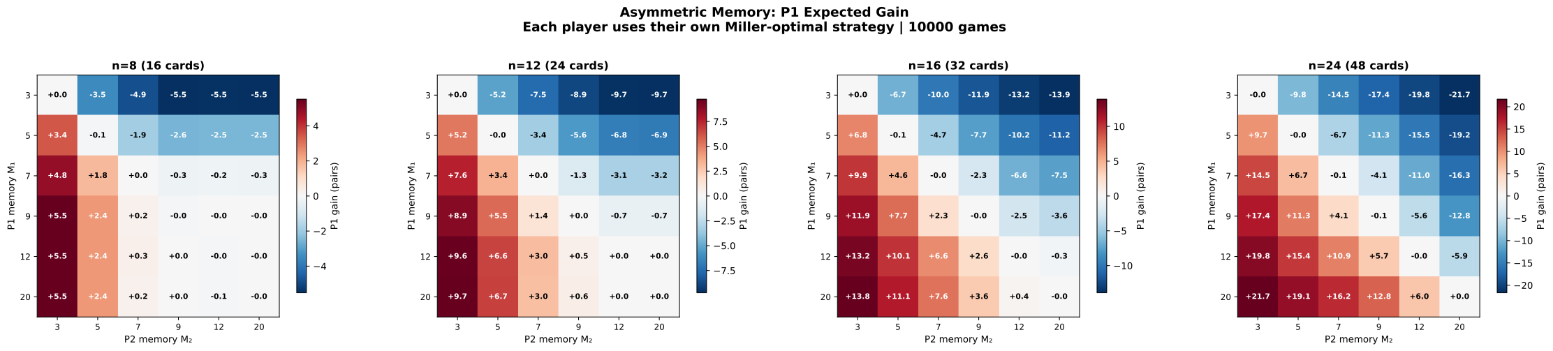
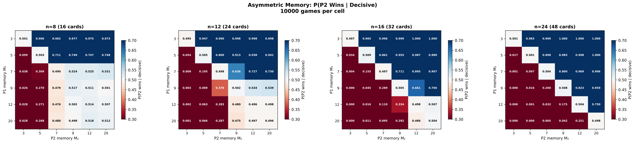
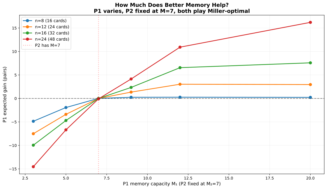
Memory capacity dwarfs positional advantage. A single extra memory slot is worth far more than the tiny first- or second-player effect.
With asymmetric memory, however, the shared-memory theorem no longer applies literally: the two players no longer have the same information state. So in that setting, these strategies should be understood as strong heuristics rather than proven optima.
8.4 Draw rate vs capacity
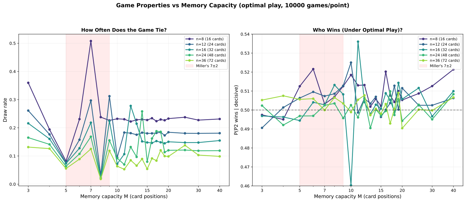
The draw rate shows a striking non-monotonic pattern. For small boards, passes can create sticky stalemates at certain capacities; once memory becomes large enough to cover the whole board, those stalemates disappear because one player eventually sweeps everything.
For standard game sizes with human-scale memory ($M\approx 7$), $M$ is far below $n$, passes typically disappear from the optimal strategy, and draws are rare.
9. Play Against the Bot
Theory is nice, but the best way to feel the difference between strategies is to play. The game below lets you play Memory against a bot that uses either the bounded-memory optimal strategy or Zwick’s perfect-recall strategy. You can adjust the bot’s memory capacity and see which cards it remembers in real time.
Try this experiment: play a few games against the bounded-memory bot ($M=7$), then switch to Zwick. With the bounded strategy, the bot flips one unknown card and keeps its memories stable. With Zwick, it flips two unknowns and old memories get evicted. The Zwick bot looks smarter because it explores faster, but on bounded memory it performs worse.
10. Code & Reproducibility
The reference implementations are all available on GitHub:
Quick Start
git clone https://github.com/taulantkoka/memory-game.git
cd memory-game
pip install numpy matplotlib joblib

# Run everything (~30 min at 100k games/point)
python run_analysis.py

# Run a single analysis
python run_analysis.py --only 01

# List available analyses
python run_analysis.py --list
11. What I Learned
- Greedy matching is optimal under shared memory: leaving a publicly known pair on the board is weakly dominated by taking it immediately.
- The bounded-memory optimum is simple: flip two new cards only at the very start; once you know a few positions, flip only one and match when you can.
- The bounded-memory strategy dominates Zwick’s on large boards, and the gap grows with size.
- Who goes first barely matters. The positional effect is real but tiny.
- What really matters is memory capacity. A single extra memory slot is worth much more than move order.
- Stalemates are mostly a perfect-memory phenomenon. Under human-scale memory limits and standard board sizes, they largely disappear.
The private-memory version of the game remains open and looks much harder: once players remember different things, the problem becomes one of incomplete information rather than perfect information.
References
- Cowan, N. (2001). The magical number 4 in short-term memory: A reconsideration of mental storage capacity. Behavioral and Brain Sciences, 24(1), 87-114.
- Miller, G. A. (1956). The magical number seven, plus or minus two: Some limits on our capacity for processing information. Psychological Review, 63(2), 81-97.
- Zwick, U., & Paterson, M. S. (1993). The memory game. Theoretical Computer Science, 110(1), 169-196.